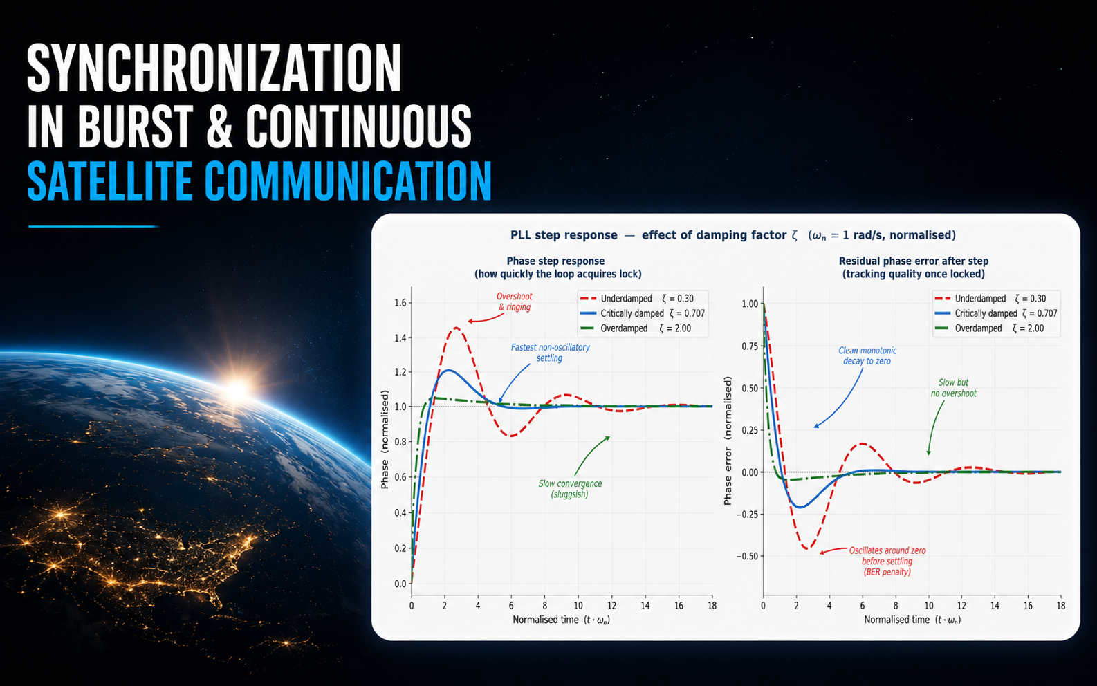
Satellite ground systems have historically been designed around one assumption: the link is continuous. Traditional LEO satellites — think the large defence, earth observation, and national programme platforms that have operated since the early space age — were built with sufficient link budget to maintain a sustained, continuous RF connection with their ground stations throughout a pass. Large antennas, high transmit power, and sensitive ground receivers gave these systems enough margin to keep the receiver locked from horizon to horizon.
NewSpace changes that assumption. The smallsats now flying in increasing numbers across commercial, defence, and national programme constellations are fundamentally link-budget-constrained. Smaller form factors mean less transmit power and smaller antennas. Lower EIRP means less margin. The practical consequence is that many of these satellites communicate in bursts: short, high-rate transmissions rather than a sustained continuous stream. Burst mode is not a design choice in the abstract; it is the direct result of operating with a tighter link budget than legacy platforms ever had to contend with.
The problem is that the ground systems serving these missions were largely built for the legacy world. Their receiver loops, modems, and operational software are optimised for continuous-mode links. Incumbent operators — national programmes, defence agencies, and earth observation operators now flying or integrating smallsats alongside their traditional platforms — are finding that their existing ground infrastructure does not handle burst-mode links reliably. The carrier recovery loop, the symbol timing loop, and the frame synchronizer all need to acquire from a cold start within a very short preamble window on every transmission, and continuous-mode receivers are simply not designed to do that.
This post documents the synchronization problem in detail: what each layer of the receiver chain needs to do, why burst mode makes it harder, and how Expedite, a modem designed with burst-mode satellite links as a first-class requirement, handles it. The practical examples throughout are drawn from our own lab work with the Satlab SRS-3, a transceiver representative of the kind of hardware now flying on exactly these link-budget-constrained smallsats.
A satellite ground station receiver does not simply look at incoming bits. Before a single bit can be decoded, the receiver must solve three separate synchronization problems: it must lock onto the carrier frequency, align its sample clock to the symbol boundaries, and find where frames begin. Get any one of these wrong and the link produces nothing, even if the RF chain is working perfectly. This post explains what each of those problems looks like, why burst-mode links make all three significantly harder, and why the seemingly mundane choice of whether to scramble your data can determine whether the link works at all.
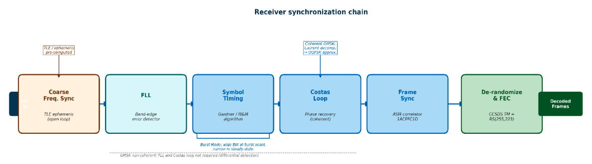
The diagram below shows the complete receiver synchronization chain, from the incoming RF signal through to decoded frames.
Why synchronization is needed
When a ground station receives a satellite downlink, the signal it sees is not a clean stream of ones and zeros. It is a band-limited, noise-corrupted, frequency-shifted analog waveform. The receiver's job is to convert that waveform back into bits, and to do that it needs to answer three questions before it can start decoding.
The first is: at what frequency is the carrier? The satellite transmitter and the ground receiver both have oscillators that are nominally at the same frequency, but they are never exactly the same. On top of oscillator imperfections, the satellite is moving, and the resulting Doppler shift moves the received carrier up or down by several kilohertz. At S-band (around 2.2 GHz), a low-Earth-orbit satellite moving at roughly 7.5 km/s can produce a Doppler shift of plus or minus 50 kHz over a pass. The receiver must find the carrier and track it as it drifts.
The second question is: where do symbols start and end? The transmitter sends symbols at a fixed rate, but the receiver has its own independent clock and has no way of knowing in advance where in time each symbol boundary falls. It must recover that timing from the received signal itself.
The third question is: where do frames begin? Even after the carrier and symbol timing are locked, the bit stream is just a sequence of bits with no obvious start point. The receiver needs to find the frame boundaries so it knows which bits belong to which field. In CCSDS-based systems this is done by sliding a correlator across the bit stream looking for the Attached Sync Marker (ASM), in our case the 32-bit pattern 1ACFFC1D.
These three problems are solved in order, because each one depends on the previous: you cannot recover symbol timing until you have the carrier frequency roughly right, and you cannot find the ASM until you have reliable symbol decisions. This ordering has real consequences for how long acquisition takes, and those consequences are most severe in burst-mode links.
The PLL: the common engine
The FLL, symbol timing recovery, and the Costas loop all share the same underlying feedback structure: the phase-locked loop (PLL). Each applies it differently — the FLL locks frequency without tracking phase, the timing loop locks the sample clock, and the Costas loop locks carrier phase — but the trade-offs of bandwidth, damping, and noise are identical in all three cases. Understanding the PLL once is the key to every loop bandwidth decision in a satellite receiver.
A second-order Type 2 PLL has three components in a feedback loop. The phase detector compares the phase of the incoming signal against the phase of a locally generated reference and produces a phase error signal. The loop filter smooths that error and shapes the loop dynamics. The VCO or NCO (numerically controlled oscillator in a digital implementation) integrates the filter output to produce the local phase reference, which feeds back to close the loop.
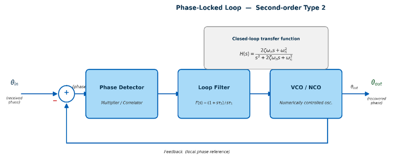
Second-order Type 2 PLL block diagram. The loop filter F(s) and the integrating VCO/NCO together give the loop its order and type. The closed-loop transfer function H(s) determines how quickly and cleanly the loop tracks the input phase.
The closed-loop transfer function is H(s) = (2ζωₙs + ωₙ²) / (s² + 2ζωₙs + ωₙ²), where ωₙ is the natural frequency (related to loop bandwidth) and ζ is the damping factor. These two parameters entirely determine the loop’s acquisition speed and steady-state tracking quality.
How ζ and ωₙ shape the response
ωₙ (natural frequency / loop bandwidth) sets the overall speed of the loop. A larger ωₙ means the loop responds faster, acquires lock more quickly, and tracks faster parameter changes, but also lets in more noise. A smaller ωₙ is quieter but slower. In the Expedite configuration, separate bandwidth parameters control the FLL, timing loop, and Costas loop independently.
ζ (damping factor) controls the character of the response within that speed. It determines whether the loop overshoots, oscillates, or sluggishly creeps toward lock. Three regimes matter in practice:
Underdamped (ζ < 1): the loop acquires quickly but overshoots and oscillates before settling. The error rings back and forth across zero, raising the bit error rate until the oscillation damps out.
Critically damped (ζ ≈ 0.707): the fastest convergence without overshoot. The error decays monotonically to zero. This is the standard design point because it minimises lock time while avoiding the BER penalty of ringing. The value ζ = 1/√2 ≈ 0.707 emerges from optimising settling time subject to the constraint of no overshoot.
Overdamped (ζ > 1): no overshoot, but the loop takes much longer to acquire. The two poles of H(s) separate along the real axis, and the slower pole dominates the settling time. For a short burst the loop may still be settling when the preamble ends, resulting in a degraded lock or missed ASM.
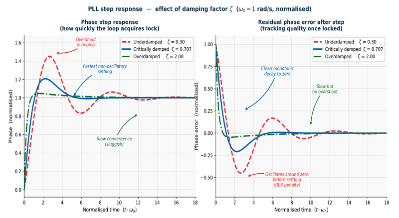
Left: phase step response showing lock speed for three damping factors. Right: residual phase error after the step. Critically damped (blue) gives the fastest non-oscillatory convergence. Underdamped (red) is fast but rings. Overdamped (green) is clean but slow.
The bandwidth / noise trade-off
The loop bandwidth sets the cut-off of the closed-loop noise transfer. Noise inside the bandwidth gets tracked by the NCO and appears in the output; noise outside is rejected. A wide loop is agile but noisy. A narrow loop is clean but slow.
In burst mode, where every loop must acquire within the preamble window, ωₙ must be wider during acquisition than in steady state. This is what the Expedite Burst Mode implements for the timing loop: it opens the bandwidth at burst onset for fast acquisition, then tightens once locked to minimise jitter during payload reception. The same trade-off applies to the FLL and Costas loop.
Frequency and phase synchronization
Frequency acquisition happens in two stages before symbol timing and phase recovery can proceed. The bulk of the Doppler error is removed open-loop from TLE ephemeris. The residual is then handled by a frequency-locked loop. Only once frequency error is small can the Costas loop lock onto the carrier phase.
Stage 1: coarse frequency correction from TLE ephemeris
The dominant source of frequency error in a LEO satellite link is Doppler shift. At S-band, a satellite moving at around 7.5 km/s produces a Doppler shift of up to approximately 50 kHz at the start and end of a pass, swinging through zero at closest approach. Rather than asking a feedback loop to acquire and track this from scratch on every burst, the receiver pre-computes the Doppler profile from the satellite TLE (Two-Line Element) ephemeris and applies it as an open-loop frequency correction before the signal reaches any feedback loop. This removes the bulk of the frequency error, leaving only the residual due to TLE age, oscillator offset, and modelling error.
Stage 2: residual frequency correction with an FLL
The residual frequency error after ephemeris correction is handled by a frequency-locked loop (FLL). An FLL is a feedback loop that drives the frequency error to zero without attempting to track phase. It is more robust to large initial frequency errors than a PLL because it does not require phase coherence to operate. The error signal is derived using a band-edge filter pair: two bandpass filters placed symmetrically around the nominal band edges of the signal. When the signal is centred correctly the energy in both filters is equal; a frequency offset tips the balance, and the difference drives the loop toward zero error. The FLL acquires over the preamble and reduces the residual offset to a level where the phase-recovery stage can take over.
The FLL loop bandwidth is set independently of the phase-recovery loop. A wider FLL bandwidth acquires the residual frequency offset faster but admits more noise into the frequency estimate. A narrower bandwidth is cleaner but slower to acquire, and will lose lock if the residual drifts faster than the loop can follow.
Symbol timing synchronization
Once the carrier is roughly correct, the receiver needs to find the symbol clock. Symbols arrive at a fixed rate from the transmitter, but the receiver samples the incoming waveform with its own independent clock. The timing recovery loop estimates the fractional offset between the transmitter symbol clock and the receiver sample clock and adjusts the sampling instants so they fall at the center of each symbol, where the eye diagram is open and the signal-to-noise ratio is highest.
Common timing error detectors include the Gardner algorithm (which works on oversampled data and is easy to implement) and the Mueller-Muller algorithm (which operates at one sample per symbol and is more noise-sensitive). Both produce a timing error signal that drives a numerically controlled oscillator to adjust the sampling phase.
The critical property that timing recovery requires is bit transitions. The timing error detector computes its estimate from the difference between adjacent samples, and if there are no transitions, the difference is always zero regardless of the sampling phase. A long run of identical bits, say a sequence of all zeros in an idle channel, produces a flat signal with no transitions and the timing loop simply drifts. This is the fundamental reason why bit transition density matters, and we will return to it when discussing scramblers.
The Timing Loop Bandwidth is the parameter that controls how quickly the timing recovery loop acquires and how much jitter it introduces in steady state. The trade-off is the same as for the carrier loop: wide bandwidth for fast acquisition, narrow bandwidth for clean steady-state tracking.
Phase recovery: the Costas loop
With frequency error removed by the FLL and symbol timing locked, the Costas loop recovers the carrier phase. The Costas loop is a PLL variant that removes the data modulation from the phase error signal — using squaring for BPSK or a decision-directed error for higher-order schemes — so the loop drives the local oscillator to the correct phase without being disrupted by data transitions. It is the Costas loop that produces the coherent phase reference the demodulator needs to project the received signal onto the correct I and Q axes.
In continuous mode, the FLL acquires at the start of a pass and hands off to the Costas loop, which tracks slow phase drift for the rest of the pass. In burst mode, both loops must acquire within the preamble window on every burst.
GMSK: a special case
Non-coherent GMSK demodulation does not require carrier recovery at all. A quadrature receiver can demodulate GMSK differentially: by comparing the phase of each symbol to the previous one rather than to an absolute reference. Because the decision is relative, oscillator phase offset cancels out. This eliminates the need for an FLL and Costas loop entirely, at a significant SNR penalty compared to coherent detection — typically around 3 dB at practical bit error rates.
Coherent GMSK demodulation recovers the full SNR advantage but requires a phase reference. The standard approach is Laurent decomposition, which shows that a GMSK signal can be expressed as a sum of amplitude-modulated pulses, the dominant term of which closely approximates an OQPSK (Offset QPSK) signal. Because OQPSK has a well-defined carrier that standard coherent techniques can lock onto, the receiver decomposes the GMSK stream using Laurent's decomposition, applies a Costas loop to the dominant OQPSK component to recover the carrier phase, and then uses that phase reference for coherent symbol detection. The approximation is tight for GMSK with BT ≥ 0.3, which covers essentially all practical satellite links including the SRS-3 at BT = 0.5.
At lower BT values (BT < 0.3), the Gaussian filter introduces more inter-symbol interference and the Laurent approximation becomes less accurate. The higher ISI means a simple matched filter no longer gives adequate performance, and an equalizer is required to recover the original symbols. A Wiener filter is the standard choice: it minimises the mean square error between the equalizer output and the transmitted symbols, taking into account both the ISI introduced by the Gaussian pulse shaping and the noise level on the channel. In practice, most satellite transceivers use BT = 0.3 or above precisely to avoid this complexity, but lower BT values do appear in bandwidth-constrained links where the spectral compactness is worth the added receiver complexity.
Frame synchronization
After symbol timing and phase recovery are locked, the demodulator is producing a stream of bits that are (mostly) correct, but the receiver still does not know where frames begin. Frame synchronization is the process of finding the ASM in the bit stream. The receiver maintains a sliding correlator that computes the Hamming distance between every 32-bit window in the bit stream and the known ASM pattern (1ACFFC1D in CCSDS systems). When the distance falls below a threshold, a frame boundary is declared and the receiver enters frame lock.
Once locked, the receiver can predict where the next ASM will appear (it is exactly one frame length away) and use that prediction to maintain lock without re-correlating every bit. It only goes back to searching if the predicted ASM is not found within a tolerance window. This makes frame sync robust once acquired, but the initial acquisition still requires the correlator to run over the entire incoming bit stream, which takes longer at lower SNR where more bit errors blur the ASM.
Frame sync is relatively straightforward in continuous mode, where the ASM appears at a predictable cadence. In burst mode, the receiver has to acquire frame sync from scratch at the start of every burst, and it needs to do so quickly enough that the ASM does not fly past before the correlator has had a chance to look.
Phase ambiguity resolution
A Costas loop has an inherent phase ambiguity. For BPSK the loop can lock at two stable points separated by π (0° and 180°), and for QPSK it can lock at four points separated by π/2. This happens because the squaring or power-of-n operation used in the Costas discriminator removes the data modulation, making the loop blind to which of the n equally-spaced lock points it has settled on. The result is that after the Costas loop acquires, the demodulator may be producing the correct bits or it may be producing a phase-rotated version of them — and there is no way to tell from the loop state alone.
The Expedite frame sync algorithm resolves this ambiguity as a by-product of ASM correlation. The correlator tests the incoming bit stream against the known ASM pattern (1ACFFC1D) in all possible phase rotations. For BPSK this means testing both the normal and bit-inverted ASM; for QPSK it means testing all four 90° rotations. Whichever rotation produces a valid ASM correlation determines the true carrier phase, and the demodulator is corrected accordingly. This means phase ambiguity resolution comes for free with frame sync — no additional mechanism is needed, and the overhead is just the extra correlator comparisons at acquisition time.
Burst mode: why it is harder
Continuous-mode communication is the easier case. The carrier loop, timing loop, and frame synchronizer all run continuously, and their only job is to track slow parameter changes (mainly Doppler drift and oscillator aging). By the time a frame arrives, all three loops are already locked.
Burst mode changes everything. The transmitter keys on, sends a burst, and keys off. The receiver sees nothing, then suddenly a signal, then nothing again. All three synchronization loops start cold at the beginning of every burst and must converge before the actual data arrives. If they do not converge in time, the data is lost.
The time available for convergence is determined by the preamble: the known sequence that precedes the payload in every burst. A longer preamble gives the loops more time to lock, at the cost of link efficiency (you are spending air time on preamble rather than payload). A shorter preamble is more efficient but puts a harder constraint on how quickly the loops must converge.
The Satlab SRS-3 is a good example of a tight constraint. Its default downlink frame begins with an 8-byte preamble (0x55 0x55 0x55 0x55 0x55 0x55 0x55 0x55). At 512 ksps that is 125 microseconds. In that window the receiver must complete AGC settling, carrier acquisition, and symbol timing acquisition, after which the ASM arrives and frame sync must lock. A conventional receiver designed for continuous-mode operation, with narrow loop bandwidths optimized for low noise in steady state, cannot do this.
How Expedite handles burst and continuous modes
Expedite is designed to operate in both modes and exposes the relevant parameters directly in the receiver configuration.
Continuous mode
In continuous mode, the Costas Loop Bandwidth and PLL Loop Bandwidth are set to values appropriate for the expected Doppler rate. The Timing Loop Bandwidth is set narrow for low jitter in steady state. There is no burst acquisition regime because the loops are always tracking. The receiver simply monitors the incoming signal and the loops run at their configured bandwidths throughout the pass. Frame sync, once acquired at the start of the pass, is maintained by prediction.
Burst mode
Burst mode is selected by checking the Burst Mode checkbox next to the Timing Loop Bandwidth field in the receiver configuration.
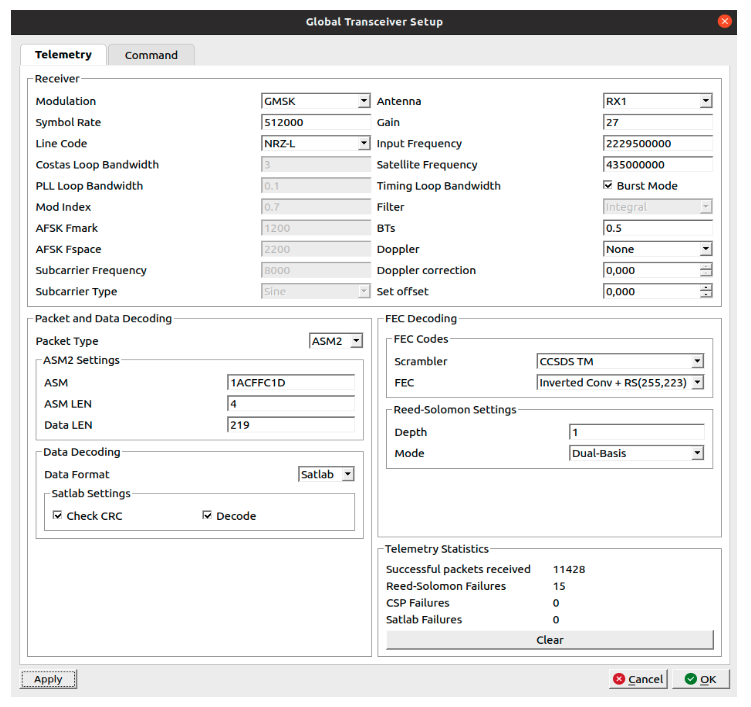
Expedite receiver configuration with Burst Mode enabled (checkbox next to Timing Loop Bandwidth). The telemetry statistics confirm 11,428 packets received with zero CSP and Satlab failures.
This does more than label the mode: it changes the behaviour of the timing recovery loop so that it uses a wider effective bandwidth at the start of each burst for fast acquisition, then tightens as lock is established. The result is that the receiver can synchronize within a very short preamble window, such as the 125-microsecond window of the SRS-3 default frame, while still achieving low jitter once locked.
Frequency and phase recovery both change in burst mode. The ephemeris Doppler correction is applied open-loop as before, but the FLL and Costas loop must each re-acquire from whatever residual offset exists at burst onset rather than tracking a continuously-locked signal. The short-term oscillator drift that accumulated while the transmitter was keyed off adds to the residual the FLL must pull in, which is one reason generous preamble length matters for burst-mode links.
On the uplink side, the Expedite transmitter uses PLOP (the CCSDS Physical Layer Operations Procedure) to give the SRS-3 receiver its own acquisition window before the data arrives. PLOP-1 prepends a CMM-2 acquisition sequence of configurable duration to each CLTU. In our SRS-3 validation we initially used 3000 ms / 2000 ms CMM2/CMM4 durations, and later reduced these to 300 ms / 200 ms with no degradation across 11,428 packets. The uplink preamble (the 8-byte 0x55 run-in in the Satlab frame settings) additionally provides the SRS-3 receiver with a transition-rich signal immediately before the ASM, complementing the PLOP acquisition sequence.
Burst mode on uplink vs downlink. The Burst Mode setting in the Expedite receiver applies to the downlink (what Expedite is receiving from the satellite). The uplink burst-acquisition challenge is on the satellite side: the SRS-3 receiver must acquire from the Expedite preamble and PLOP acquisition sequence. These are separate problems with separate solutions, both present in the same link.
Scramblers, randomizers, and why bit transition density matters
We mentioned earlier that timing recovery needs bit transitions. This is not a minor concern. In a real satellite link, there are many situations where long runs of identical bits can appear: idle channels, telemetry frames where most fields are zero, padding, or simply data that happens to have low entropy for a particular pass. When these runs are long enough, the timing loop loses its reference and drifts. By the time transitions reappear, the sampling phase may have moved far enough from the symbol center that bit errors increase sharply.
The solution is to randomize the data before transmission so that long runs are broken up regardless of the original content. This is what the CCSDS pseudo-randomizer does. It XORs every bit of the frame (after the ASM, which must remain unmodified for the frame synchronizer) with a deterministic pseudorandom sequence generated by the polynomial:
CCSDS TM: h(x) = x^8 + x^7 + x^5 + x^3 + 1 (initialized to 0xFF)
CCSDS TC: h(x) = x^8 + x^6 + x^4 + x^3 + x^2 + x + 1 (initialized to 0xFF)
G3RUH: h(x) = 1 + x^12 + x^17
The sequence generated by this polynomial has maximum length (it visits every possible state before repeating) and is balanced: over a full period, it contains nearly equal numbers of zeros and ones. XORing a data stream with this sequence converts any long run into a pseudorandom pattern with frequent transitions. The receiver generates the same sequence in synchrony and XORs again to recover the original data. Because the sequence is deterministic and both sides initialize to the same state (0xFF) at the start of each frame, no side information is needed.
It is worth being clear about what scrambling does and does not do. It does not encrypt the data. Someone who knows the polynomial and the initialization state can de-randomize the stream just as the intended receiver does. The purpose is purely to ensure spectral and transition properties: the randomized stream has a more uniform power spectrum (no discrete spectral lines from repeated patterns), fewer long runs of identical bits, and a guaranteed minimum transition density that the timing and carrier loops can rely on.
Scrambler types supported by Expedite
Expedite supports three scramblers, selectable in the FEC Codes section: CCSDS TM, CCSDS TC, and G3RUH (multiplicative). Understanding the difference between them matters because the transmitter and receiver must use the same type, and choosing the wrong one produces a de-randomized bit stream that looks plausible but is entirely wrong.
CCSDS TM and CCSDS TC are both additive scramblers. An additive scrambler works by XORing the data stream with a pseudo-random sequence generated by a linear feedback shift register (LFSR). Because XOR is its own inverse, the receiver applies the identical sequence to recover the original data. The scrambler and de-scrambler are the same circuit. CCSDS TM uses the polynomial h(x) = x⁸ + x⁷ + x⁵ + x³ + 1, initialized to 0xFF, and is applied to the frame payload after the ASM. CCSDS TC uses h(x) = x⁸ + x⁶ + x⁴ + x³ + x² + x + 1, also initialized to 0xFF, and operates on the CLTU structure of the uplink command channel. Neither scrambler touches the synchronization markers, which must remain unscrambled for the frame synchronizer to find them.
G3RUH is a multiplicative (self-synchronising) scrambler. Rather than XORing with an independent LFSR sequence, G3RUH feeds the data bits back through the shift register: the scrambled output depends on both the current input bit and the previous scrambled bits. The polynomial is h(x) = 1 + x¹² + x¹⁷ (see the original G3RUH circuit diagram for the LFSR implementation). Because the scrambler state is derived from the data itself, a multiplicative scrambler is self-synchronising: if the receiver loses sync and then re-acquires it, the de-scrambler re-locks within a number of bits equal to the shift register length, without needing a frame-level reset. The trade-off is that a single bit error in the received stream propagates into multiple errors at the de-scrambler output (error multiplication), whereas an additive scrambler passes bit errors through one-for-one. G3RUH is common in amateur satellite and some low-cost commercial downlinks.
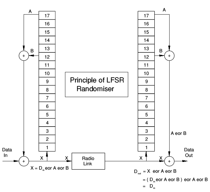
Expedite selects the scrambler in the FEC Codes section. The choice must match the satellite. The CCSDS TM scrambler is the standard for CCSDS-compliant telemetry downlinks and was used in our SRS-3 validation. On the receiver side, the de-randomizer runs after frame sync is declared, before Reed-Solomon decoding. The ordering matters: the frame synchronizer must find the ASM in the unscrambled bit stream (the ASM itself is never scrambled), and the RS decoder must operate on de-scrambled data.
One subtlety is the interaction with the inner convolutional code. The convolutional encoder runs after the randomizer, so the Viterbi decoder on the receive side runs before the de-randomizer. The de-randomized bits feed directly into the RS decoder. If the de-randomizer is out of sync by even one bit, the RS decoder sees what looks like a burst of errors across the entire codeword, usually more than the 16-symbol correction capacity of RS(255,223), and the frame fails. This is why frame synchronization must be reliable before the de-randomizer is started.
What happens without a scrambler
A useful way to understand why scrambling matters is to consider what happens without it. An all-zero idle frame, for example, produces a constant signal after modulation with no transitions. The timing recovery loop, deprived of edges to lock onto, drifts freely. The carrier loop also suffers: for MSK-family modulations the carrier phase is carried by the transitions between symbols, and without transitions the phase reference degrades.
In practice, most links that operate without scrambling rely on the data itself to provide enough transitions. Compressed telemetry, encrypted payloads, and sensor data typically have high entropy and will naturally produce frequent transitions. But relying on data entropy is fragile: it works until the data happens to be low-entropy, which is exactly when you cannot afford a synchronization failure. The scrambler eliminates this dependence and guarantees transition density regardless of what the payload contains.
For the same reason, the preamble bytes are chosen as 0x55 (alternating ones and zeros in binary) rather than, say, 0x00 or 0xFF. Alternating bits produce a maximum-transition-density sequence that the timing and carrier loops can lock onto in the shortest possible time. This is why both the CCSDS PLOP acquisition sequence and the Satlab uplink preamble use this pattern.
Putting it together
The three synchronization problems and the scrambling requirement are not independent. They form a chain, and each link depends on the previous one. Carrier lock enables symbol timing recovery. Symbol timing recovery requires transitions (hence the scrambler and the preamble pattern). Symbol timing recovery enables reliable bit decisions. Reliable bit decisions enable ASM correlation and frame sync. Frame sync enables de-randomization. De-randomization enables RS decoding.
In continuous mode, this chain is established once at the start of a pass and maintained throughout. The loops only need to be fast enough to acquire from a standing start, and after that they run in steady-state tracking mode for the duration.
In burst mode, the chain must be re-established on every burst, within the time budget allowed by the preamble. This requires wider loop bandwidths for fast acquisition, a preamble pattern that is maximally useful for the loops (0x55), and a receiver architecture that is explicitly designed for burst operation. The Expedite Burst Mode is exactly this: a receiver that widens its timing loop bandwidth at burst onset, acquires within the short preamble window, and tightens back down for payload tracking, all transparently.
The SRS-3 validation we published earlier is a concrete example of all of this in action. The 8-byte SRS-3 preamble, the CCSDS scrambler, the Burst Mode setting on the Expedite receiver, and the PLOP acquisition sequence on the uplink are each solving one part of the synchronization problem for a short-burst S-band link. Understanding why each setting is there makes it much easier to diagnose what is wrong when a new link does not work on the first attempt.
References
CCSDS 131.0-B-3, TM Synchronization and Channel Coding
CCSDS 401.0-B, Radio Frequency and Modulation Systems
End-to-End Validation of the Expedite Modem with the Satlab SRS-3